The theory理论

The mathematics of Siyuan Code思源码的数学

A self-contained account of the bijective coding, the Trie automaton, and the counting algorithm — the formal problem, the optimality argument, and every definition, theorem and algorithm that makes it work.关于双射编码、Trie 自动机与计数算法的自洽阐述——形式化问题、最优性论证，以及让它成立的每一个定义、定理与算法。

1 · Formal problem1 · 形式化问题

Too-long strands are expensive and inaccurate, so the information is cut into parts of length $n$. Let the information alphabet be $\mathcal{A}=\{0,1\}$ and the DNA alphabet $\mathcal{B}=\{A,T,C,G\}$. An encoding is any mapping from binary strings of length $n$ to DNA strings; $\mathrm{len}(\cdot)$ is the string-length function.

过长的链既昂贵又易错，因此信息被切成长度为 $n$ 的小段。设信息字母表为 $\mathcal{A}=\{0,1\}$，DNA 字母表为 $\mathcal{B}=\{A,T,C,G\}$。编码就是任意一个从长度 $n$ 的二进制串到 DNA 串的映射；$\mathrm{len}(\cdot)$ 是串长函数。

$$ f:\mathcal{A}^n \to \mathcal{B}^* $$

Definition · Suitable strand定义 · 可用链

A DNA sequence is suitable if and only if:一条 DNA 序列 可用（suitable） 当且仅当：

no homopolymer longer than $k$;
没有长度超过 $k$ 的同聚物；
GC content within $[\mathrm{GC}_{\min}, \mathrm{GC}_{\max}]$;
GC 含量落在 $[\mathrm{GC}_{\min},\mathrm{GC}_{\max}]$ 内；
no undesired motif.
不含任何不良基序。

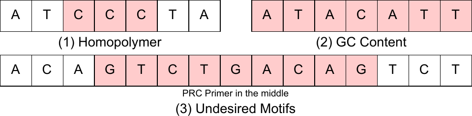
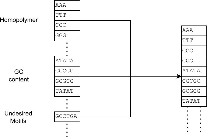
Rules (1) and (2) are themselves just undesired motifs: rule (1) adds every $(k{+}1)$-fold repetition of a base, and rule (2) adds every short window whose local GC content leaves the allowed range. So a single set $\mathcal{I}$ of “bad” substrings captures all three rules, and a strand is unsuitable exactly when it contains some $u\in\mathcal{I}$ as a substring. $S_k$ is the set of suitable strands of length $k$, and $\mathcal{S}_k=\bigcup_{i=1}^{k}S_i$.

规则 (1)(2) 本身也只是不良基序：规则 (1) 加入每种碱基的 $(k{+}1)$ 连重复，规则 (2) 加入所有局部 GC 含量越界的短窗口。于是单个"坏"子串集合 $\mathcal{I}$ 就统一刻画了三条规则，一条链不可用当且仅当它包含某个 $u\in\mathcal{I}$ 作为子串。$S_k$ 是长度 $k$ 的可用链集合，$\mathcal{S}_k=\bigcup_{i=1}^{k}S_i$。

Error patterns — Supplementary Fig.The three error patterns.三类错误模式。

Building additional motifs — Supplementary Fig.Homopolymer and GC rules encoded as motifs.同聚物与 GC 规则被编码为基序。

1.1 · GC content is controlled by the law of large numbers1.1 · GC 含量由大数定律控制

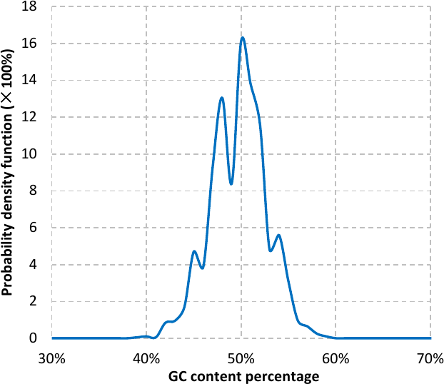
Local GC content is constrained directly (every length-5 window must stay in range). Global GC content is instead left to the law of large numbers: a random strand concentrates near 50%. The following theorem bounds how rare an extreme global GC is.

局部 GC 含量被直接约束（每个长度 5 的窗口都必须在范围内）。全局 GC 含量则交给大数定律：随机链会集中在 50% 附近。下面的定理给出极端全局 GC 有多罕见的上界。

Theorem · Rareness of global GC error定理 · 全局 GC 误差的罕见性

Let $s\in\mathcal{B}^n$, and let $X$ be the fraction of positions whose base is in $\{C,G\}$. Then设 $s\in\mathcal{B}^n$，$X$ 为碱基落在 $\{C,G\}$ 的比例。则 $\mathrm{Var}(X)=\dfrac{1}{4n}$.

Proof证明$\mathbb{E}(X)=\frac12$, and by independence $\mathrm{Var}(X)=\frac{1}{n^2}\cdot n\,\mathrm{Var}(X_i)=\frac{1}{4n}$. Approximating by a normal distribution,$\mathbb{E}(X)=\frac12$，由独立性 $\mathrm{Var}(X)=\frac{1}{n^2}\cdot n\,\mathrm{Var}(X_i)=\frac{1}{4n}$。用正态分布近似， $$ P(|X-0.5|>c) \approx 2\,\mathrm{CDF}(-2c\sqrt{n}). $$ At $n=100$, $P(|X-0.5|>0.15)\approx 0.0027$ — well within what error correction absorbs at negligible cost.取 $n=100$，$P(|X-0.5|>0.15)\approx 0.0027$——远小于纠错以极低成本即可覆盖的范围。

GC content distribution — Supplementary Fig.Measured GC distribution: 99% of strands fall within 42.9–57.6%.实测 GC 分布：99% 的链落在 42.9–57.6%。

1.2 · The input is uniform after compression1.2 · 压缩后输入是均匀的

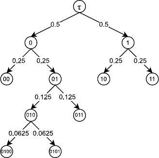
Density is defined against a uniform input, and this is justified: if a file were not uniform, an optimal Huffman code would compress it further. By the optimality of Huffman coding and Jensen's inequality,

密度是相对均匀输入定义的，这有依据：若文件不均匀，最优 Huffman 编码还能进一步压缩它。由 Huffman 编码的最优性与 Jensen 不等式，

$$ \mathbb{E}_{X\sim p}[\mathrm{len}(hc(X))] \le H(X)+1 = \mathbb{E}[-\log_2 p(X)]+1 \le \mathrm{len}(x)+1, $$

with equality only when $p$ is uniform. A non-uniform compressed file is therefore, by definition, not optimally compressed.

等号仅在 $p$ 均匀时取到。因此压缩后仍不均匀的文件，按定义就没有被最优压缩。

Supplementary Fig.An ideal Huffman tree, where each split is balanced.理想 Huffman 树：每次分裂左右权重相等。

2 · Density and optimality2 · 密度与最优性

Definition · Density定义 · 密度

$$ d(f)=\frac{\mathbb{E}_x[\mathrm{len}(x)]}{\mathbb{E}_x[\mathrm{len}(f(x))]}, \qquad d(T)=\frac{n}{\mathbb{E}_x[\mathrm{len}(T(x))]}\le 2. $$ Since $|\mathcal{B}|=4$, two bits per nucleotide is the hard ceiling.因为 $|\mathcal{B}|=4$，每个核苷酸 2 比特是硬上限。

The set of suitable strands grows geometrically: $\lim_{i\to\infty}|S_{i+1}|/|S_i|\in(2,4)$. Let $T'_{k,n}$ be the one-to-one mapping from $\mathcal{A}^n$ onto the set $\mathcal{S}_k$ of suitable strands of length at most $k$, and $T_{k,n}$ the one-to-one mapping onto the set $S_k$ of suitable strands of exactly length $k$. Two facts follow.

可用链集合按几何级数增长：$\lim_{i\to\infty}|S_{i+1}|/|S_i|\in(2,4)$。设 $T'_{k,n}$ 是从 $\mathcal{A}^n$ 到长度不超过 $k$ 的可用链集合 $\mathcal{S}_k$ 的一一映射，$T_{k,n}$ 是从 $\mathcal{A}^n$ 到长度恰为 $k$ 的可用链集合 $S_k$ 的一一映射。有两个结论。

Lemma引理

The variable-length code set is contained in one more length:变长码集可以被多一位的定长码集容纳： $$ |\mathcal{S}_k|=\sum_{i=1}^{k}|S_i| \le |S_{k+1}|\cdot\Big(\tfrac12+\tfrac14+\tfrac18+\cdots\Big) < |S_{k+1}|. $$

Theorem · Uniform length is as good定理 · 定长同样好

$$ \lim_{k\to\infty} d(T'_k) - \lim_{k\to\infty} d(T_k) = 0. $$

Proof证明The gap is the round-off of one length:差距只是一个长度的取整： $$ \lim_{k\to\infty}\Big(\frac{n}{k}-\frac{n}{k+1}\Big) = \lim_{k\to\infty}\frac{n}{k(k+1)} = 0. $$

So a fixed-length code — one number per strand — reaches the same limit. Concretely, sort $S_k$ in lexicographic order and map the integer $i$ to the $(i{+}1)$-th smallest strand. This is the whole of bijective coding. It is optimal:

因此定长编码——每条链一个编号——达到同样的极限。具体做法：把 $S_k$ 按字典序排序，把整数 $i$ 映射到第 $(i{+}1)$ 小的链。这就是双射编码的全部。它是最优的：

Theorem · Optimality定理 · 最优性

$T'$ is optimal: no encoding exceeds density$T'$ 是最优的：任何编码的密度都无法超过 $\lim_{k\to\infty}\dfrac{\log_2|\mathcal{S}_k|}{k}$.

Proof · by contradiction证明 · 反证 Suppose a better encoding $f:\mathcal{A}^n\cup\mathcal{A}^{n-1}\cup\cdots\cup\mathcal{A}^1\to\mathcal{S}_k$ had higher density, $\lim_k d(f)>\lim_k \log_2|\mathcal{S}_k|/k$. Then假设存在更好的编码 $f:\mathcal{A}^n\cup\mathcal{A}^{n-1}\cup\cdots\cup\mathcal{A}^1\to\mathcal{S}_k$ 有更高密度，$\lim_k d(f)>\lim_k \log_2|\mathcal{S}_k|/k$。那么 $$ \lim_{k\to\infty} d(f)=\lim_{k\to\infty}\frac{\mathbb{E}_x[\mathrm{len}(x)]}{k}\ \ge\ \lim_{k\to\infty}\frac{\log_2|\mathcal{S}_k|}{k}\,(1+\epsilon). $$ Hence for some $k$ and input $x$,于是对某个 $k$ 与输入 $x$， $$ |\mathcal{A}^n\cup\mathcal{A}^{n-1}\cup\cdots\cup\mathcal{A}^1|\ \ge\ 2^{\mathrm{len}(x)}\ \ge\ 2^{(\log_2|\mathcal{S}_k|)(1+\epsilon)}\ >\ |\mathcal{S}_k|\,(1+\epsilon). $$ The number of distinct inputs exceeds the number of strands, so two inputs must map to the same strand and $f$ cannot be decoded correctly — contradiction.不同输入的个数超过了链的个数，于是两个输入必然映射到同一条链，$f$ 无法正确解码——矛盾。

This is why the method is called density-optimal: the bijection reaches the exact information-theoretic ceiling of the constrained channel, not a heuristic bound. The same logic explains our density accounting: $405.8$ EB/g without redundancy, $246.7$ EB/g after index, checksum and error correction, and $41$ EB/g once the six physical copies are counted — the honest, apples-to-apples number.

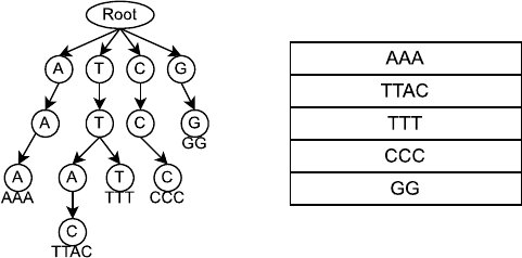
这正是它被称为 密度最优 的原因：双射达到该约束信道的精确信息论天花板，而非启发式上界。同样的逻辑解释了我们的密度核算：无冗余 $405.8$ EB/g，计入索引、校验与纠错后 $246.7$ EB/g，再计入 6 份物理拷贝为 $41$ EB/g——即公平可比的诚实数字。

3 · The Trie3 · Trie 树

Enumerating all $4^k$ strands is impossible — the suitable set grows exponentially. The key observation is the reverse: the unsuitable set is small. Instead of storing the exponentially many good strands, we store the few bad patterns in a trie — a tree whose root-to-node paths spell the prefixes of $\mathcal{I}$.

枚举全部 $4^k$ 条链不可行——可用集合指数增长。关键在于反过来：不可用集合很小。与其存储指数多的好链，不如把为数不多的坏模式存进一棵 trie——它的根到节点路径拼出 $\mathcal{I}$ 的前缀。

$$ V=\{\,v \mid \exists u\in\mathcal{I},\ v \text{ is a prefix of } u \,\}. $$

Lemma · Construction引理 · 构造

The trie is built in $O(L)$ time and space, where $L=\sum_{u\in\mathcal{I}}\mathrm{len}(u)$ is the total length of the constraint set. (Standard, and used — not proposed — here.)trie 可在 $O(L)$ 时间与空间内建成，其中 $L=\sum_{u\in\mathcal{I}}\mathrm{len}(u)$ 是约束集的总长。（这是经典结论，此处是使用而非提出。）

A strand is read base by base; after each base, the buffer is a growing prefix of the strand. The crucial reduction: a strand contains an unsuitable substring iff, at some step, the longest suffix of the buffer that is a trie node lies in $\mathcal{I}$.

链逐碱基读入；每读一个碱基，缓冲区都是该链不断增长的前缀。关键归约：链包含不可用子串，当且仅当在某一步，缓冲区在 trie 中的 最长后缀 落在 $\mathcal{I}$ 里。

Theorem · Detecting an unsuitable strand定理 · 判定不可用链

$v$ contains a substring in $\mathcal{I}$ $\iff$ some prefix $w$ of $v$ has a suffix in $\mathcal{I}$ $\iff$ the longest suffix of $w$ that is in $V$ lies in $\mathcal{I}$.$v$ 含 $\mathcal{I}$ 中的子串 $\iff$ $v$ 的某个前缀 $w$ 有后缀在 $\mathcal{I}$ 中 $\iff$ $w$ 在 $V$ 中的最长后缀落在 $\mathcal{I}$ 里。

Proof证明 A strand is read base by base; after each base the buffer $w$ is a growing prefix of the strand, and the strand contains a motif iff some buffer prefix has a suffix in $\mathcal{I}$:链逐碱基读入；每读一个碱基，缓冲区 $w$ 都是该链不断增长的前缀。链含基序，当且仅当某个缓冲区前缀有落在 $\mathcal{I}$ 中的后缀： $$ v\text{ unsuitable}\ \iff\ \exists\, w\in\mathrm{prefix}(v),\ \exists\, u\in\mathcal{I}: u\in\mathrm{suffix}(w). $$ Let $u'$ be the longest suffix of $w$ that is a trie node. (1) Any $u\in\mathcal{I}$ that is a suffix of $w$ is a suffix of $u'$ — since $u'$ is the longest suffix of $w$ in $V$ and $\mathcal{I}\subseteq V$ — hence $u'$ contains a motif and lies in $\mathcal{I}$. (2) Conversely, if a proper suffix of $u'$ were in $\mathcal{I}$, then $u'$, containing it, would also be in $\mathcal{I}$. So the condition is exactly $u'\in\mathcal{I}$.设 $u'$ 为 $w$ 在 trie 中的最长后缀。(1) 任何作为 $w$ 后缀的 $u\in\mathcal{I}$ 必是 $u'$ 的后缀——因为 $u'$ 是 $w$ 在 $V$ 中的最长后缀、且 $\mathcal{I}\subseteq V$——故 $u'$ 含基序、自身落在 $\mathcal{I}$ 中。(2) 反过来，若 $u'$ 的某个真后缀在 $\mathcal{I}$ 中，则含它的 $u'$ 也应在 $\mathcal{I}$ 中。因此条件恰为 $u'\in\mathcal{I}$。

Corollary推论

So checking suitability reduces to tracking, at every step, the longest buffer suffix that is a trie node. A naive check costs $O(L)$ per step — $O(nL)$ overall — which is polynomial but too slow. The next section accelerates it to $O(n)$.因此可用性判定归结为：每步跟踪缓冲区在 trie 中的最长后缀。朴素检查每步 $O(L)$——总共 $O(nL)$——多项式但太慢。下一节把它加速到 $O(n)$。

Supplementary Fig.The trie of unsuitable patterns.不良模式的 trie。

4 · AC algorithm and the Trie automaton4 · AC 算法与 Trie 自动机

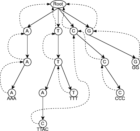
The Aho–Corasick (AC) automaton accelerates longest-suffix tracking with a fail edge $F$: the longest proper suffix of a node that is still a trie node. After appending a character $c$, one walks fail edges until a node with an outgoing $c$ is found.

Aho–Corasick（AC）自动机用 失败边（fail edge） $F$ 加速最长后缀跟踪：一个节点的最长真后缀、且仍是 trie 节点。追加字符 $c$ 后，沿失败边走，直到找到有 $c$ 出边的节点。

$$ F(v)=\arg\max_{u\in V,\ u\ne v,\ u\in \mathrm{suffix}(v)}\mathrm{len}(u). $$

Supplementary Fig.The classical AC automaton and its fail edges.经典 AC 自动机及其失败边。

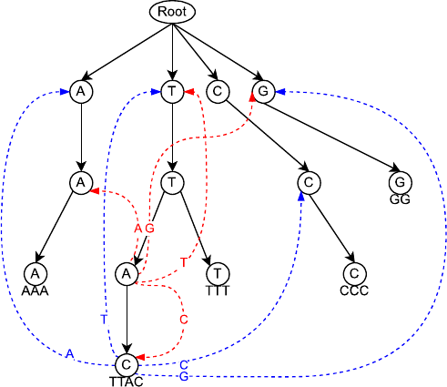
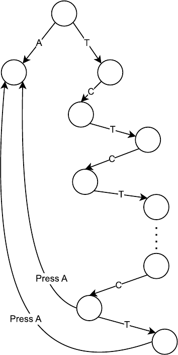
AC guarantees amortized $O(1)$ per step — enough for pattern matching, which scans each character once. Encoding does not scan: it must randomly access every successor of every node to count and choose, which breaks the amortization. We therefore replace the fail-edge walk with a precomputed press edge $P_c(v)$, the longest suffix of $v{+}c$ in $V$ — a single direct transition, so every step is strict worst-case $O(1)$.

AC 保证每步摊还 $O(1)$——这对"每个字符只扫一次"的模式匹配够了。但编码不是扫描：它必须 随机访问每个节点的所有后继 来计数与选择，这会破坏摊还。于是我们用预计算的 按压边（press edge） $P_c(v)$——即 $v{+}c$ 在 $V$ 中的最长后缀——取代失败边回退，一步直达，因此每步都是 严格最坏情况 $O(1)$。

$$ P_c(v)=\arg\max_{u\in V,\ u\in \mathrm{suffix}(v+c)}\mathrm{len}(u). $$

The press and fail edges are computed together in one BFS pass:

按压边与失败边在一次 BFS 中一并算出：

$$ P_c(v{+}c')=\begin{cases} \mathrm{child}_c(v{+}c') & \text{if } \mathrm{child}_c(v{+}c') \text{ exists}\\ P_c(F(v{+}c')) & \text{otherwise} \end{cases} $$ $$ P_c(\mathrm{root})=\begin{cases} c & \text{if } \mathrm{child}_c(\mathrm{root}) \text{ exists}\\ \mathrm{root} & \text{otherwise} \end{cases}, \qquad F(v{+}c')=P_{c'}(F(v)) \ \ (v\ne\mathrm{root}), \qquad F(\mathrm{root})=F(c')=\mathrm{root}. $$

Theorem · Well-definedness定理 · 良定义

The formulas are well-defined: each right-hand side is computed before it is used, in BFS order.这些公式是良定义的：按 BFS 顺序，每个右端在使用前都已算好。

Proof证明 By definition $\mathrm{len}(P_c(v{+}c'))\le \mathrm{len}(v{+}c')+1$ and $\mathrm{len}(F(v{+}c'))\le \mathrm{len}(v{+}c')-1$. Computing by BFS, when we reach $v{+}c'$ the press and fail edges of every string no longer than $\mathrm{len}(v)$ are already computed; $F(v)$ is known with $\mathrm{len}(F(v))\le n'-1$, so $P_{c'}(F(v))$ is known, hence $P_c(P_{c'}(F(v)))$ is known — the right-hand sides are available.按定义 $\mathrm{len}(P_c(v{+}c'))\le \mathrm{len}(v{+}c')+1$ 且 $\mathrm{len}(F(v{+}c'))\le \mathrm{len}(v{+}c')-1$。按 BFS 计算到 $v{+}c'$ 时，所有不长于 $\mathrm{len}(v)$ 的串的 press/fail 边都已算好；$F(v)$ 已知且 $\mathrm{len}(F(v))\le n'-1$，故 $P_{c'}(F(v))$ 已知，进而 $P_c(P_{c'}(F(v)))$ 已知——右端齐备。

Theorem · Correctness定理 · 正确性

The defined edges are the intended longest suffixes in $V$.所定义的边正是 $V$ 中应有的最长后缀。

Proof证明 (1) On one hand $P_{c'}(F(v))$ is a suffix of $v{+}c'$ shorter than $v{+}c'$, so it is no longer than $F(v{+}c')$. On the other hand $\mathrm{par}(F(v{+}c'))$ is a suffix of $v$ shorter than $v$, so it is no longer than $F(v)$, giving $\mathrm{len}(F(v{+}c'))=\mathrm{len}(P_{c'}(\mathrm{par}(F(v{+}c'))))\le \mathrm{len}(P_{c'}(F(v)))$. Thus $F(v{+}c')=P_{c'}(F(v))$.(1) 一方面 $P_{c'}(F(v))$ 是 $v{+}c'$ 的一个更短后缀，故不长于 $F(v{+}c')$。另一方面 $\mathrm{par}(F(v{+}c'))$ 是 $v$ 的一个更短后缀，故不长于 $F(v)$，于是 $\mathrm{len}(F(v{+}c'))=\mathrm{len}(P_{c'}(\mathrm{par}(F(v{+}c'))))\le \mathrm{len}(P_{c'}(F(v)))$。故 $F(v{+}c')=P_{c'}(F(v))$。 (2) If $\mathrm{child}_c(v{+}c')$ exists the result is trivial. Otherwise $P_c(v{+}c')$ is no longer than $v{+}c'$: on one hand $P_c(F(v{+}c'))$ is a suffix of $v{+}c'{+}c$, hence no longer than $P_c(v{+}c')$; on the other hand $\mathrm{par}(P_c(v{+}c'))$ is a shorter suffix of $v{+}c'$, hence no longer than $F(v{+}c')$, giving $\mathrm{len}(P_c(v{+}c'))=\mathrm{len}(P_c(\mathrm{par}(P_c(v{+}c'))))\le \mathrm{len}(P_c(F(v{+}c')))$. Thus $P_c(v{+}c')=P_c(F(v{+}c'))$.(2) 若 $\mathrm{child}_c(v{+}c')$ 存在则显然。否则 $P_c(v{+}c')$ 不长于 $v{+}c'$：一方面 $P_c(F(v{+}c'))$ 是 $v{+}c'{+}c$ 的后缀，故不长于 $P_c(v{+}c')$；另一方面 $\mathrm{par}(P_c(v{+}c'))$ 是 $v{+}c'$ 的更短后缀，故不长于 $F(v{+}c')$，于是 $\mathrm{len}(P_c(v{+}c'))=\mathrm{len}(P_c(\mathrm{par}(P_c(v{+}c'))))\le \mathrm{len}(P_c(F(v{+}c')))$。故 $P_c(v{+}c')=P_c(F(v{+}c'))$。

Trie-automaton constructionTrie 自动机构造

preprocess press, fail for root and its children
for v in BFS order of V (v ≠ root):
  for c′ in {A,T,C,G} where child_c′(v) exists:
    v′ ← child_c′(v)
    fail[v′] ← press_c′[ fail[v] ]
    for c in {A,T,C,G}:
      press_c[v′] ← child_c(v′) if it exists, else press_c[ fail[v′] ]

Longest-suffix tracking with press edges用按压边跟踪最长后缀

s ← root
for c in Str:
  s ← press_c[s]          # one step, strict O(1)
  append s to Suffix[]

Theorem · Complexity定理 · 复杂度

Construction takes $O(L)$ time and $O(L)$ space; tracking takes $O(n)$ time and $O(n)$ space.构造 $O(L)$ 时间、$O(L)$ 空间；跟踪 $O(n)$ 时间、$O(n)$ 空间。

Trie automaton with press edges — Supplementary Fig.The automaton with fail and press edges.带失败边与按压边的自动机。

Amortization failure — Supplementary Fig.A case where the classical AC algorithm's amortized $O(1)$ degrades to $O(L)$ per step under the encoding access pattern — the motivation for the strict-$O(1)$ press edge.在编码访问模式下，经典 AC 算法的摊还 $O(1)$ 退化到每步 $O(L)$ 的例子——这正是引入严格 $O(1)$ 按压边的动机。

5 · Dynamic-programming counting5 · 动态规划计数

Theorem · Unsuitable ⟺ the press path visits $\mathcal{I}$定理 · 不可用 ⟺ 按压路径经过 $\mathcal{I}$

$$ s=(s_1,\dots,s_n)\text{ unsuitable} \iff \exists i,j:(s_i,\dots,s_j)\in\mathcal{I} \iff \{\tau,\,P_{s_1}(\tau),\,P_{s_2}(P_{s_1}(\tau)),\dots\}\cap\mathcal{I}\ne\emptyset. $$ So a suitable strand is exactly a press-edge path that never visits $\mathcal{I}$.因此可用链恰好是一条从不经过 $\mathcal{I}$ 的按压边路径。

Definition · $\mathrm{DP}$定义 · $\mathrm{DP}$

Let $\mathrm{DP}(v,l)$ be the number of suitable paths of length $l$ starting from node $v$.设 $\mathrm{DP}(v,l)$ 为从节点 $v$ 出发、长度为 $l$ 的可用路径数。

Theorem · Recurrence定理 · 递推

$$ \mathrm{DP}(v,0)=\begin{cases} 0 & v\in\mathcal{I}\\ 1 & v\notin\mathcal{I} \end{cases}, \qquad \mathrm{DP}(v,l)=\begin{cases} \sum_{c\in\mathcal{B}}\mathrm{DP}(P_c(v),\,l-1) & v\notin\mathcal{I}\\ 0 & v\in\mathcal{I} \end{cases}. $$

Proof证明 The boundary is the empty path: $\mathrm{DP}(v,0)=1$ iff $v$ itself is suitable. For $l>0$, a suitable path of length $l$ from $v$ decomposes uniquely into pressing a first base $c$, then a suitable path of length $l-1$ from $P_c(v)$. Summing over the four first bases counts every path exactly once:边界是空路径：$\mathrm{DP}(v,0)=1$ 当且仅当 $v$ 本身可用。对 $l>0$，从 $v$ 出发的长度 $l$ 可用路径唯一分解为"先按压首碱基 $c$，再从 $P_c(v)$ 走长度 $l-1$ 的可用路径"。对四种首碱基求和即不重不漏： $$ \mathrm{DP}(v,l)=\sum_{c\in\mathcal{B}}\mathrm{DP}(P_c(v),\,l-1). $$ Whether $P_c(v)$ is suitable is irrelevant: if $P_c(v)\in\mathcal{I}$, then $\mathrm{DP}(P_c(v),\,l-1)=0$ by the boundary, so the sum is unaffected.$P_c(v)$ 是否可用无关紧要：若它在 $\mathcal{I}$ 中，则由边界条件 $\mathrm{DP}(P_c(v),\,l-1)=0$，求和不受影响。

To account for the primers, the boundary is revised: $\mathrm{DP}(v,0)=0$ if adding any prefix of the reverse primer from $v$ lands in $\mathcal{I}$, and $1$ otherwise. The transition is unchanged — so every emitted strand stays suitable through both primers.

为计入引物，边界被修订：若从 $v$ 出发加上反向引物的任一前缀会落入 $\mathcal{I}$，则 $\mathrm{DP}(v,0)=0$，否则为 $1$。递推不变——于是每一条输出的链在加上两个引物后仍然可用。

Theorem · DP complexity定理 · DP 复杂度

The $\mathrm{DP}$ table is built in $O(nL)$ time and space.$\mathrm{DP}$ 表在 $O(nL)$ 时间与空间内建成。

DP value calculation (with primer revision)DP 值计算（含引物修订）

for v in V:
  ok ← True; u ← v
  if u ∈ I: ok ← False
  for c in primerR: u ← P_c(u); if u ∈ I: ok ← False
  DP[v,0] ← 1 if ok else 0
for l = 1 … n:
  for v in V:
    DP[v,l] ← 0 if v ∈ I else Σ_{c∈{A,T,C,G}} DP[P_c(v), l-1]

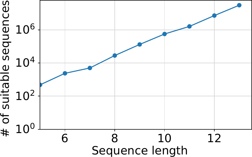
Number of suitable strands grows exponentially — Supplementary Fig.The number of suitable strands grows exponentially (≈ $3.783^n$) — the space the bijection fully exploits.可用链数量随长度指数增长（约 $3.783^n$）——双射所充分挖掘的空间。

6 · Encoding and decoding6 · 编码与解码

Encoding maps an integer $i$ to the $(i{+}1)$-th lexicographically smallest suitable strand. Choosing the first base is a counting decision: walk the bases in order, and take the first branch whose count exceeds what remains.

编码把整数 $i$ 映射到字典序第 $(i{+}1)$ 小的可用链。选择第一个碱基就是一个计数决策：按序遍历碱基，取第一个"剩余计数"够大的分支。

$$ \mathrm{Enc}(v,i,l) = c + \mathrm{Enc}\!\Big(P_c(v),\ i-\sum_{d<c}\mathrm{DP}(P_d(v),\,l-1),\ l-1\Big). $$

Encode — the $i$-th suitable strand of length $L$编码 — 第 $i$ 条长度为 $L$ 的可用链

v ← P_primerL(root)
for j = 0 … L−1:
  depth ← L − j − 1
  for c in {A,T,C,G}:
    if i < DP[P_c(v)][depth]:   # this branch contains strand i
      emit c; v ← P_c(v); break
    else:
      i ← i − DP[P_c(v)][depth]

Decoding is the mirror image: count how many suitable strands are lexicographically smaller than the given strand.

解码是其镜像：数出比给定链字典序更小的可用链有多少。

$$ \mathrm{Dec}(v,s) = \sum_{c<s_1}\mathrm{DP}(P_c(v),\,j-1) + \mathrm{Dec}(P_{s_1}(v),\,s'), \qquad s'=(s_2,\dots,s_j). $$

Decode — the ordinal of a given strand解码 — 给定链的序号

i ← 0; v ← P_primerL(root)
for j = 0 … L−1:
  depth ← L − j − 1
  for c in {A,T,C,G}:
    if c = Strand[j]: v ← P_c(v); break
    else: i ← i + DP[P_c(v)][depth]
return i

Theorem · Encode correctness定理 · 编码正确性

The algorithm outputs the $(i{+}1)$-th lexicographically smallest suitable strand.算法输出字典序第 $(i{+}1)$ 小的可用链。

Proof证明 Conquer recursively. At a node $v$, try $c_0$ first. If $i$ is smaller than $\mathrm{DP}(P_{c_0}(v),\,l-1)$, the number of suitable strands starting with $c_0$, then the first base is $c_0$ and the rest is $\mathrm{Enc}(P_{c_0}(v),\,i,\,l-1)$. Otherwise the target lies in a later branch: subtract $\mathrm{DP}(P_{c_0}(v),\,l-1)$ from $i$ and try $c_1$, and so on.递归分治。在节点 $v$ 先试 $c_0$。若 $i$ 小于以 $c_0$ 开头的可用链数 $\mathrm{DP}(P_{c_0}(v),\,l-1)$，则首碱基为 $c_0$、其余为 $\mathrm{Enc}(P_{c_0}(v),\,i,\,l-1)$。否则目标在更靠后的分支：把 $i$ 减去 $\mathrm{DP}(P_{c_0}(v),\,l-1)$ 再试 $c_1$，以此类推。

Theorem · Decode correctness定理 · 解码正确性

The algorithm returns the number of suitable strands lexicographically smaller than the given strand.算法返回比给定链字典序更小的可用链数。

Proof证明 Split the strands smaller than $s=(s_1,\dots,s_j)$ into two parts: those whose first base $c$ is smaller than $s_1$, and those sharing the first base $s_1$. The former contribute $\sum_{c<s_1}\mathrm{DP}(P_c(v),\,j-1)$; the latter are counted recursively by $\mathrm{Dec}(P_{s_1}(v),\,s')$, where $s'=(s_2,\dots,s_j)$.把小于 $s=(s_1,\dots,s_j)$ 的链分成两部分：首碱基 $c<s_1$ 的，与首碱基同为 $s_1$ 的。前者贡献 $\sum_{c<s_1}\mathrm{DP}(P_c(v),\,j-1)$；后者由 $\mathrm{Dec}(P_{s_1}(v),\,s')$ 递归计数，其中 $s'=(s_2,\dots,s_j)$。

Theorem · Complexity定理 · 复杂度

Encoding and decoding a single strand each take $O(n)$ time and $O(n)$ space; the $O(nL)$ $\mathrm{DP}$ preprocessing is shared across strands and amortizes away.单链编码与解码各耗时 $O(n)$、空间 $O(n)$；$O(nL)$ 的 $\mathrm{DP}$ 预处理在所有链间共用、被摊还掉。

Proof证明 Each algorithm runs an outer loop of $n$ iterations with a constant-size inner loop, so $O(n)$ time. The $\mathrm{DP}$ table (built once, in $O(nL)$) is read, not rebuilt, for every strand.每个算法都是 $n$ 次外层循环、常数大小的内层循环，故 $O(n)$ 时间。$\mathrm{DP}$ 表只建一次（$O(nL)$），每条链只读不重建。

7 · Error correction7 · 纠错系统

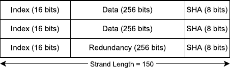
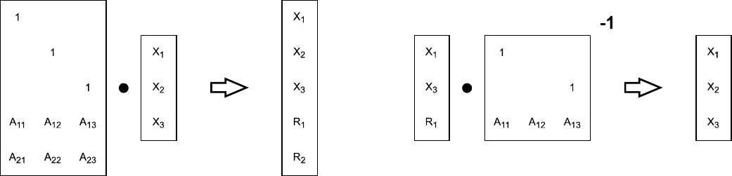
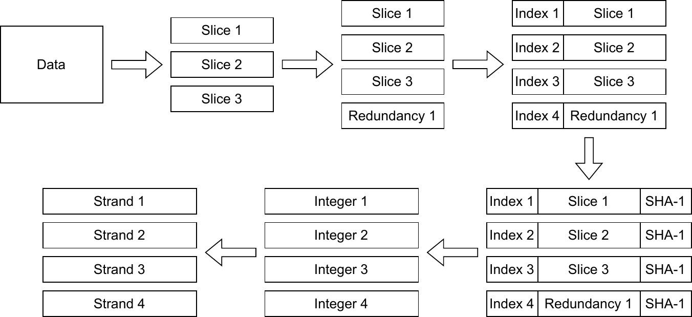
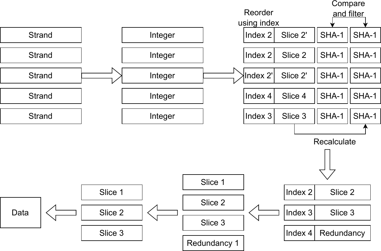
The bijective core is wrapped into a full codec. A file is cut into slices, and each slice gets an index to recover its order after sequencing, and a checksum (high bits of SHA-1) for intra-slice detection. A Reed–Solomon erasure code adds parity slices for inter-slice correction.

双射核心被封装成完整编解码器。文件切成片，每片带索引以在测序后恢复顺序、带 校验和（SHA-1 高位）用于片内检测；Reed–Solomon 删除码加入 校验片 用于片间纠错。

Slicing — Supplementary Fig.Slice structure: data + index + checksum.切片结构：数据 + 索引 + 校验。

7.1 · Why inter-slice, not intra-slice7.1 · 为什么片间、而非片内纠错

Intra-slice correction would need the error-transition probability $\Pr(\text{errored }t \mid \text{source }s)$, which biology does not supply:

片内纠错需要误差转移概率 $\Pr(\text{出错为 }t \mid \text{源 }s)$，而生物学并不提供它：

$$ Err(s,t)=\Pr(\text{errored data is } t \mid \text{source is } s), \qquad \arg\max_x \Pr(x)\,Err(x,y). $$

Across slices, however, errors are symmetric and independent — exactly the setting erasure codes were built for. RS parity is added to the data before indices, so it does not disturb the encoding, and each parity slice carries its own index and checksum.

但跨切片时，误差对称且独立——这正是删除码所设计的场景。RS 校验在加索引之前加到数据上，因此不干扰编码；每片校验也自带索引与校验和。

7.2 · Intra-slice detection and multi-time sequencing7.2 · 片内检测与多次测序

The checksum lets each read be judged correct in isolation, so error correction only ever deals with known-good or known-missing slices. Sequencing each strand multiple times and keeping the hash-verified reads drives the single-strand error probability down exponentially.

校验和让每次读取能被单独判定是否正确，于是纠错只需处理"已知正确"或"已知缺失"的片。每条链多次测序、只保留通过校验的读取，使单链错误概率呈指数下降。

Encoding pipeline — Supplementary Fig.Encoding: slice → RS parity → index → checksum → strand.编码：切片 → RS 校验 → 索引 → 校验和 → 链。

Decoding pipeline — Supplementary Fig.Decoding: filter by checksum, order by index, correct by RS.解码：按校验过滤、按索引排序、按 RS 纠错。

8 · Complexity8 · 复杂度

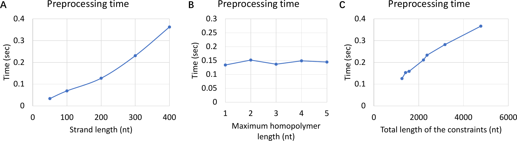
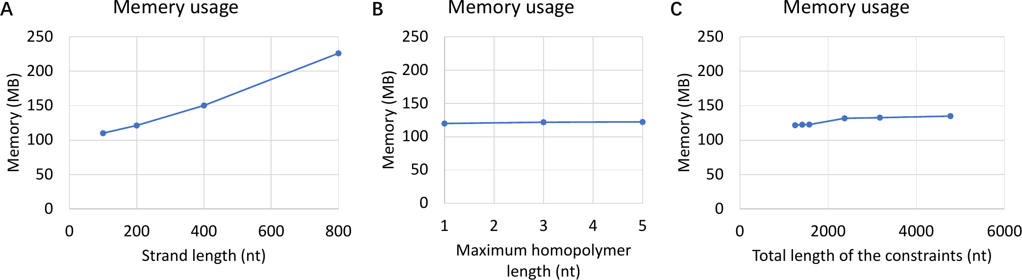
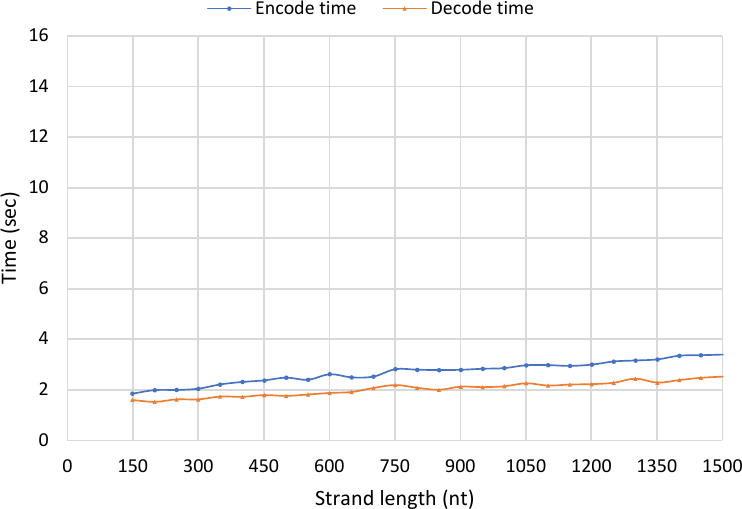
Here $n$ is the strand length, $L$ the total length of the constraint set, and $L_{\text{file}}$ the file size. The cost is independent of how strict the constraints are.

这里 $n$ 是链长，$L$ 是约束集总长，$L_{\text{file}}$ 是文件大小。成本与约束多严格无关。

Stage阶段	Time时间	Space空间
Trie automatonTrie 自动机	$O(L)$	$O(L)$
DP countingDP 计数	$O(nL)$	$O(nL)$
Encode / decode (one strand)编码/解码（单链）	$O(n)$	$O(n)$
Encode / decode (whole file)编码/解码（整文件）	$O(L_{\text{file}})$	$O(L_{\text{file}})$

Theorem · Whole-file complexity定理 · 整文件复杂度

Encoding or decoding an entire file takes $O(L_{\text{file}})$ time: there are $O(L_{\text{file}}/n)$ strands, each costing $O(n)$.编码或解码整个文件耗时 $O(L_{\text{file}})$：共有 $O(L_{\text{file}}/n)$ 条链，每条 $O(n)$。

Supplementary Fig.Preprocessing time scales linearly with strand length and constraint length.预处理时间随链长与约束长度线性增长。

Preprocessing space — Supplementary Fig.Preprocessing memory scales linearly as well.预处理内存同样线性增长。

Long strands — Supplementary Fig.For strands far beyond 300 nt, the running time grows only gradually — the cost does not depend on constraint strictness.即便链长远超 300 nt，运行时间也只缓慢增长——成本不随约束严格程度而变。

Prefer the plain-language version?想看通俗版？ Read the intuition →阅读直觉 →

Stage阶段	Time时间	Space空间
Trie automatonTrie 自动机	\(O(L)\)	\(O(L)\)
DP countingDP 计数	\(O(nL)\)	\(O(nL)\)
Encode / decode (one strand)编码/解码（单链）	\(O(n)\)	\(O(n)\)
Encode / decode (whole file)编码/解码（整文件）	\(O(L_{\text{file}})\)	\(O(L_{\text{file}})\)